Building a Local Semantic Search Engine - Part 2: From Keywords to Meaning

This is Part 2 of a series on building a local semantic search engine. Read Part 1 for an introduction to embeddings.

Traditional search fails when you don't remember the exact words. Searching "debugging" won't find your notes about "fixing bugs." Semantic search finds them anyway—because it searches by meaning, not keywords.

The magic is cosine similarity—a way to measure how "alike" two embedding vectors are. It returns a score from 0 to 1, where higher means more similar.

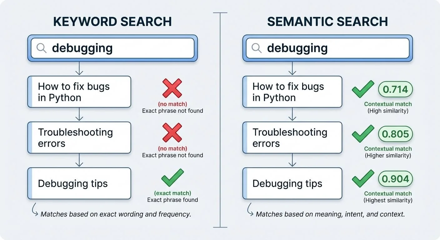
Keyword vs semantic search: Semantic search finds related documents even with different words

The implementation is straightforward (semantic_search.py:43-47):

def cosine_similarity(vec1, vec2):
    v1 = np.array(vec1)
    v2 = np.array(vec2)
    return np.dot(v1, v2) / (np.linalg.norm(v1) * np.linalg.norm(v2))

That's it. Dot product divided by magnitudes. The math is simple; the results feel like mind-reading.

These rough thresholds are common starting points (codified in demo_lmstudio.py):

• 0.80+: Very similar, likely about the same thing
• 0.60-0.80: Good match, related topics
• 0.40-0.60: Weak match, tangentially related
• Below 0.40: Very different, probably unrelated

To search, I embed the query, then calculate similarity against every document's embedding. Sort by score, return the top results (semantic_search.py:167-191):

def search(query, index, top_k=5):
    query_embedding = get_embedding(query)
    results = []
    for doc in index["documents"]:
        similarity = cosine_similarity(query_embedding, doc["embedding"])
        results.append((doc, similarity))
    results.sort(key=lambda x: x[1], reverse=True)
    return results[:top_k]

Note that doc["embedding"] comes from a pre-computed cache—document embeddings are generated once during indexing and stored in a JSON file. Only the query embedding is computed at search time. This means the first indexing run is slow, but subsequent searches are fast since they just load embeddings from disk and do simple math. The tradeoff: it's a linear scan through all chunks, which works fine for hundreds of documents but would need a proper vector database for thousands. (We'll dive deeper into caching in Part 4.)

Similarity scores aren't binary—they're a gradient. A 0.58 match might be exactly what you're looking for, or noise. Context matters.

Semantic search has known limitations: exact matches, code symbols, and proper nouns. If you search "ValueError," you want files with that exact string, not conceptually similar error types. For deeper coverage of these tradeoffs, see Pinecone's guide to semantic search. The best approach combines keyword and semantic search.

Next: indexing a whole directory and the chunking strategy that makes it work.

---

Part 2 of 5 in the EmbeddingGemma series.

---

embeddinggemma - View on GitHub

---

This post is part of my daily AI journey blog at Mosaic Mesh AI. Building in public, learning in public, sharing the messy middle of AI development.